Human-LLM text segmentation on M1 Max: WCP works, raw log-likelihood doesn't
 Contents
A new paper came out that, given a piece of text where human-written and LLM-written sentences are mixed, tries to estimate sentence by sentence where the writer switched.
arXiv:2605.03723, “Segmenting Human-LLM Co-authored Text via Change Point Detection,” posted on May 5, 2026, licensed under CC BY 4.0.
As far as I could check, no official implementation by the authors is bundled on the arXiv page or in the TeX source.
Reproducing the same experiment as the paper requires AdaDetectGPT, FastDetectGPT, a Gemma 2 9B-class scoring model, the CoAuthor dataset, and pre-generated mixed documents.
But the core of the method — applying change point detection to a sequence of “LLM-likeness” scores — can be tried in fairly small Python.
Like the paper on warmth-tuned LLMs becoming more agreeable and the paper on fine-tuning increasing verbatim copying of books, this isn’t about a crude binary “did an LLM write this or not.”
The problem is that real-world text is already mixed. A human writes the body, an LLM adds captions for tables and figures, the human edits again.
Slapping an “AI-generated” label on the entire document at that point is too coarse to be useful.
Naive per-sentence scoring lets boundaries jump around
The paper’s idea is straightforward.
Split the text into a sequence of sentences X1, X2, ... XN, and attach an LLM detection score phi(Xi) to each.
If the score tends to be low for human sentences and high for LLM sentences, the score series looks like time series data.
Find where the mean shifts abruptly, and you’re close to where the author changed.
There are weaknesses in classifying sentence by sentence directly.
First, the threshold is hard to fix.
A boundary like “score ≥ 0.6 means LLM” moves with dataset, model, style, and sentence length.
The other issue is short sentences.
Scores like FastDetectGPT compute statistics from next-token probabilities.
Short sentences have few observations, so they’re noisy.
Long sentences are relatively stable.
Treating every sentence with equal weight means a single short noisy sentence can spawn a boundary.
The paper brings change point detection — point estimation of where a series mean changes — into this picture.
Specifically, it adopts the Narrowest-Over-Thresholding (NOT) family to pick multiple boundaries from the sentence-level score series.
The proposed methods come in three flavors: VCP, WCP, and GCP.
VCP is plain CUSUM, WCP is CUSUM weighted by per-sentence reliability, and GCP applies the detector to entire concatenated regions instead of averaging sentence-level scores.
Weighted CUSUM doesn’t overtrust short sentences
The intuition behind WCP is clean.
If longer sentences give more stable detection scores, weight them higher.
The paper’s theoretical recipe uses the inverse of each score’s variance as the weight.
In practice, you can use estimated variance, or use a power of token count as a proxy.
I started with a synthetic test: no detector, just CUSUM with hand-made scores.
Make the first 5 sentences “human-like” (low) and the next 5 “LLM-like” (high), with sentence lengths as weights.
from math import sqrt

scores = [0.13, 0.18, 0.11, 0.16, 0.20, 0.72, 0.81, 0.77, 0.86, 0.79]
lengths = [18, 14, 22, 11, 19, 34, 42, 37, 45, 39]

def weighted_cusum(y, w, s, e, b):
    left_w = sum(w[s:b + 1])
    right_w = sum(w[b + 1:e + 1])
    total_w = left_w + right_w

    left_mean = sum(w[i] * y[i] for i in range(s, b + 1)) / left_w
    right_mean = sum(w[i] * y[i] for i in range(b + 1, e + 1)) / right_w

    return sqrt(left_w * right_w / total_w) * abs(left_mean - right_mean)

values = [
    (b + 1, weighted_cusum(scores, lengths, 0, len(scores) - 1, b))
    for b in range(len(scores) - 1)
]

print(values)
print(max(values, key=lambda item: item[1]))
The output:
[(1, 2.07), (2, 2.71), (3, 3.82), (4, 4.26), (5, 4.92), (6, 4.08), (7, 3.02), (8, 2.46), (9, 1.26)]
(5, 4.92)
The maximum is “after sentence 5.”
Exactly the synthetic boundary.
Of course, this isn’t testing an LLM detector’s quality.
What it tests is the part the paper centers on: turning a sentence-level score series into a boundary estimate.
For multiple boundaries, you don’t apply CUSUM once over the whole sequence.
You sample candidate intervals randomly, take the shortest one whose CUSUM exceeds the threshold, and recurse left and right.
That’s the NOT-style processing.
The paper uses M=200 and roughly sqrt(log(N)) for the threshold.
Reproducing the full experiment is heavy on a home machine
The main experiment uses 100 documents each of WikiQA, News, and Story, replacing parts of human documents with GPT-5-mini or Claude 4.5 to construct mixed documents.
Evaluation metrics are WindowDiff and Count Error.
Baselines include per-sentence classification, Voting, TextTiling, asking an LLM directly to predict boundaries, and PaLD.
The detection scores are AdaDetectGPT, FastDetectGPT, log-likelihood, and log-likelihood log-rank ratio.
For FastDetectGPT-family scores, the paper uses google/gemma-2-9b-it as the scoring model.
The hardware is an H20 96GB GPU with 96 Xeon Platinum 8255C CPU cores.
Reading this far, reproducing the paper’s tables on a Mac or a normal gaming PC is at least not light work.
That said, the heavy part of the experiment isn’t change point detection — it’s generating sentence-level LLM detection scores at scale.
Change point detection alone runs on standard Python.
For a small test, the realistic path is to pick one existing LLM detector, dump per-sentence scores to a CSV, and run WCP on that column.
Tested with Qwen3-8B-Base on M1 Max
The paper uses Gemma 2 9B + FastDetectGPT/AdaDetectGPT.
I didn’t have Gemma 2 9B locally, so I substituted Qwen3-8B-Base, which I already had cached.
Instead of FastDetectGPT, I use raw avg log-likelihood directly.
This drifts from the paper’s main experiment, but it’s enough to see whether the lightweight version of the implementation comes together.
I load Qwen3-8B-Base via HF transformers and run it on the MPS backend.
For each sentence I call model(ids, labels=ids) and read off avg log-likelihood.
The resulting series is z-standardized and fed to WCP + NOT.
The threshold is sqrt(log N), the same as the paper.
I prepared two inputs.
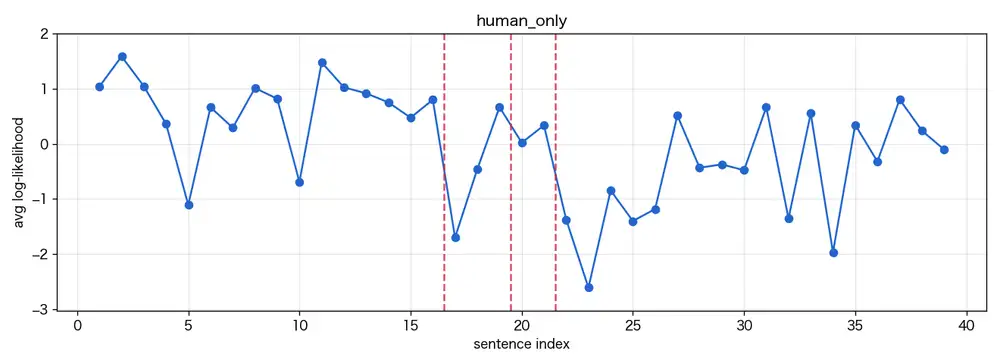
The human-only text is the first two pages of one of my own self-published novels in Japanese (39 sentences).
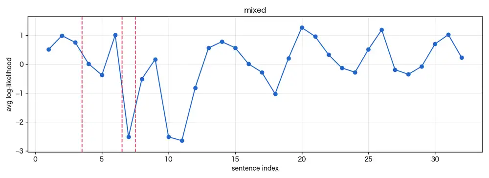
The mixed text is one of my own blog posts (LLM draft, manually edited and rewritten by me, 32 sentences).
The human-only text starts with the narrator (a teacher) musing in monologue and ends with a student barging into the staff room.
The first half is descriptive narration, the second is short dialog.
The human-only run produced 21 raw candidates.
Taking the top 3 by CUSUM, boundaries fell after sentences 16, 19, and 21.
The maximum was 12.6.
The shift after sentence 19 is especially clear.
19: そう、たまにはこういう平穏な日があってもいい、たとえ仕事が何もなくても、
    どうせ古書部の面々が何かしらの事件を持ち込んできて、いつも私の至福のまどろみを邪魔するのだから。
20: 「せんせーせんせーくませんせー!」
21: そうそう、こんなふうに。
That’s the moment the narrator’s internal monologue switches to a student calling out.
It’s natural for the detector to react there.
The mixed text produced 13 raw candidates, with the top 3 falling after sentences 3, 6, and 7.
Maximum CUSUM was 3.0.
The article is about playing with Google Flow to dress up an original character in different costumes — intro → procedure → image comments → impressions, an ordinary blog structure.
The boundaries landed around the procedural list.
5: 使ったのはウェブ版のGeminiとGoogle Flowだけ。
6: Geminiに衣装を着ている画像を入れて「人物を消して衣装だけにして、背景は単色で」
7: と指示
8: 大体これ一発で衣装だけになる
Short fragments using nominal endings (体言止め in Japanese) line up there.
This doesn’t correspond to a human/AI switch point.
Why it reacted there is a limitation of the method, discussed below.
How to read “AI-likeness” from the graph
The y-axis is the per-sentence avg log-likelihood, z-standardized.
Higher values (towards positive) mean the sentence is easier for Qwen to predict; lower means more surprising.
LLMs select high-probability sequences when generating, so even a different LLM scoring those tends to find them predictable.
A region where AI wrote consecutively should show up as a plateau pinned near the top of the graph.
The left and right edges of that plateau correspond to where the AI region starts and ends, and that’s what CUSUM picks up — the textbook scenario.
In practice this plateau is barely visible.
The human-only text (my own novel) has scores swinging widely between -2 and -7, but that’s not a plateau, it’s oscillation.
Long monologue sentences are predictable and float to the top, while short shouted dialog drops to the bottom.
What the swings reflect isn’t who wrote the text — it’s just style and sentence length.
CUSUM reaches 12.6 because the mean difference between the chunk of narration and the chunk of dialog is large.
If a human writes for a while in one style and then switches to another, plenty of “boundaries” rise inside that single document.
The mixed text (LLM-drafted blog post that I edited) swings the same way but with smaller amplitude.
The narrator’s tone has been smoothed out across the article, so an “AI-like” plateau, if it ever existed, doesn’t show up on the graph.
Short fragments of one or two tokens (Japanese 体言止め endings like “と指示”) become outliers, and CUSUM clings to those instead.
Given this kind of oscillation, you can’t read “this part is AI” from the raw-score graph directly.
The paper uses FastDetectGPT or AdaDetectGPT to suppress, by construction, the variance contributed by sentence length and style — only after that does a “plateau on top” become a usable AI signature.
With raw scores, that prerequisite doesn’t even hold.
Even a calibrated score doesn’t always give a clean answer.
Sentences a human polished into AI-like form, or AI output that a human heavily rewrote, will have the plateau partially erased.
The mixed text I tested is exactly the latter case: the editing pass flattened the plateau, leaving the small-amplitude graph that came out.
GCP looks promising but multiplies scoring calls
GCP, instead of averaging per-sentence scores, applies the detector to the concatenated text of the left region and the right region directly.
A region as a whole gives the detector a longer input, more stable than looking at short sentences one by one.
The reasoning is quite natural.
The cost is more compute.
NOT recursively examines many intervals, so GCP calls the detector each time.
That’s fine if the detector is a small statistic, but with a 9B model it gets heavy fast.
For a small experiment, reusing the score series with WCP is more workable.
Treat detected boundaries as candidates, not evidence
This method isn’t a tool to declare AI use.
The paper itself frames the problem as “localizing human-LLM co-authored text” — finer-grained than slapping a label on a document, but still dependent on the input detection score.
LLM detectors waver on style, genre, language, translation, polishing, and paraphrasing.
Some sentences are humans polished into LLM-like form; others are LLM output a human heavily edited.
The paper’s CoAuthor experiment uses three classes (human / collaborative / LLM-generated), but only because that data was made in a logged editor where ground-truth labels are available.
If you’re using this in practice, the output reads more like “a writer or generation step might have changed here” — review candidates.
It’s not something to apply directly to disciplinary decisions on student papers or workplace documents.
Used alongside edit history, generation logs, and citation checking — as supporting evidence for reading mixed documents — the approach plays well.
References
- arXiv:2605.03723 Segmenting Human-LLM Co-authored Text via Change Point Detection
- Creative Commons Attribution 4.0 International
- arXiv:2403.03506 Detecting AI-Generated Sentences in Realistic Human-AI Collaborative Hybrid Texts — Zeng et al. (IJCAI 2024). A different family of methods that this paper cites — sequence labeling with SegFormer-style models for per-sentence AI/human classification. Implementation at douglashiwo/AISentenceDetection, though this is not the official code for the paper covered in this post.